SAS to R Notes
How I did part of a SAS assignment in R
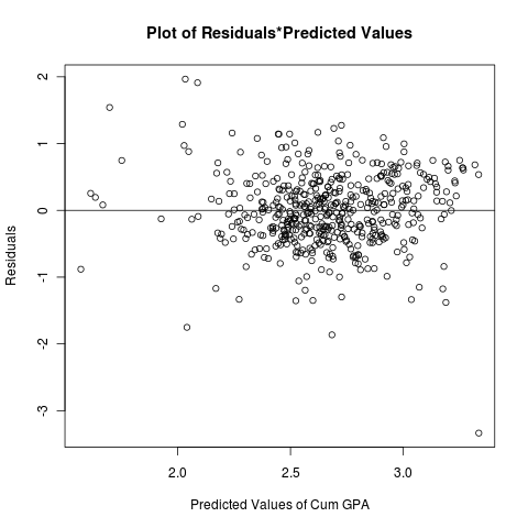
I was working on a SAS assignment for my Regression Analysis class. The residual plot in SAS was corrupted, luckily I was able to recreate it in R. (And actually it looks better in R too.)
# read in data from file
gpa.data <- read.table("GPA.txt");
# create multiple linear regression model
gpa.fit <- lm(V4 ~ V1 + V2 + V3 + V5 + V6 + V7 + V8, data=gpa.data)

# save residuals to a variable
gpa.resid <- residuals(gpa.fit)
# save Predicted values to a variable
gpa.yhat <- fitted.values(gpa.fit)

# create png file, that plot will be saved to.
#png("resid.png")
# create a plot of residuals vs predicted values
plot(gpa.yhat,gpa.resid, ylab="Residuals", xlab="Predicted Values of Cum GPA", main="Plot of Residuals*Predicted Values")
# create a line#
abline(0,0)
# write plot to file
#dev.off()

ANOVA table of the Multiple Regression Model
Here is R's ANOVA command. Run it on the regression model gpa.fit.
Here is the output of the ANOVA command.
The stars in R's output are the signoificance code. In the above
summary output, V2, V3, V5 are very significant. V1, V7, and V8 are
not very significant; the regression model should be tested without them.
anova(gpa.fit)
Analysis of Variance Table

Response: V4
           Df  Sum Sq Mean Sq F value    Pr(> F)
V1          1   0.567  0.5669  1.8709  0.172001
V2          1  26.488 26.4877 87.4135 < 2.2e-16 ***
V3          1   9.096  9.0964 30.0194 6.839e-08 ***
V5          1   2.446  2.4459  8.0717  0.004683 **
V6          1   1.032  1.0324  3.4069  0.065524 .
V7          1   0.020  0.0199  0.0655  0.798068
V8          1   0.278  0.2784  0.9187  0.338288
Residuals 492 149.084  0.3030
---
codes:  0 ‘***’ 0.001 ‘**’ 0.01 ‘*’ 0.05 ‘.’ 0.1 ‘ ’ 1
Summary of Linear Regression Model
summary(gpa.fit)
Call:
lm(formula = V4 ~ V1 + V2 + V3 + V5 + V6 + V7 + V8, data = gpa.data)

Residuals:
    Min      1Q  Median      3Q     Max
-3.3345 -0.3387 -0.0059  0.3429  1.9661

Coefficients:
              Estimate Std. Error t value Pr(> |t|)
(Intercept)  1.7792451  0.5165056   3.445  0.00062 ***
V1          -0.0383924  0.0527532  -0.728  0.46710
V2           0.2716557  0.0417213   6.511 1.84e-10 ***
V3           0.0010404  0.0003173   3.279  0.00111 **
V5           0.0010332  0.0003425   3.016  0.00269 **
V6          -0.0391177  0.0239319  -1.635  0.10279
V7          -0.0006554  0.0028471  -0.230  0.81805
V8          -0.0054118  0.0056462  -0.958  0.33829
---
codes:  0 ‘***’ 0.001 ‘**’ 0.01 ‘*’ 0.05 ‘.’ 0.1 ‘ ’ 1

Residual standard error: 0.5505 on 492 degrees of freedom
Multiple R-squared: 0.2112, Adjusted R-squared:   0.2
F-statistic: 18.82 on 7 and 492 DF,  p-value: < 2.2e-16